Table of Contents

1. Introduction
2. The Problem with Implied Volatility
3. Understanding Black-Scholes Inversion
4. Existing Root Finding Approaches
5. The GCM-H Algorithm: Combining Known Techniques

LINK TO PAPER

---

Introduction

This past semester, I've been taking a numerical analysis course where we focused on a lot of interesting topics, the most engaging of which I found to be root-finding algorithms. For my final project, we were tasked with conducting research in the field of numerical analysis and, with my interest in finance, I started exploring the applications of root finding algorithms to options volatility calculations. After doing some reading, I came to the important realization that the goal of developing new and faster root-finding (or any) algorithms isn't always about creating universally superior methods, but rather developing techniques that excel within specific problem domains imposing specific limitations. With options pricing calculations, such limitations are plentiful. With this in mind, I decided to try and piece together another root finding algorithm that is specifically tailored towards the challenges that come along with options volatility calculations.

In this post, I try to explain my approach with theory and reasoning. The paper is attached. Please note that I am still a student with no real industry experience, so remember that while I am attempting to create a novel approach, this project is more of a learning experience for myself than a legitimate attempt at a novel contribution. According to what I've been able to find online, I assume that, to tackle this particular problem, an informed quantitative researcher at a real firm would lean towards something like Peter Jackel's "Let's Be Rational", or some proprietary variant. Similar to how computer science students often implement a linux shell from scratch to learn how a shell works, I hope that this project is conducive to my goal of building a strong foundation in quantitative research.

For the options pricing layman, here are the basic ideas:

1. Options are contracts representing the right to buy (or sell) a security in the future at a specified price.

2. Options traders don't always think in terms of dollar prices, they think in terms of implied volatility. When you see an option trading at one dollar, what traders actually care about is "what volatility assumption makes the Black-Scholes model output one dollar?"

3. This creates an inverse problem: given the market price, solve backwards to find the implied volatility.

4. Why does this matter? For market making and risk management in options, quants need to calculate implied volatilities across a lot of options simultaneously which allows them to compute important things like risk exposure every time the market moves, and (for market makers) quote fresh bid/ask prices in real-time.

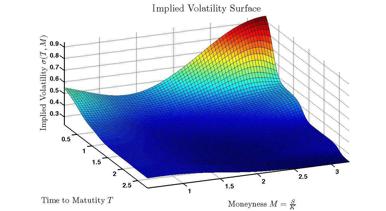
5. The computational challenge is that this inverse problem becomes numerically unstable for certain types of options (specifically, deep out-of-the-money options). Standard algorithms either fail or become very slow in these cases.

6. In this project, I combine several existing techniques into a single algorithm that handles these problematic cases more efficiently, reducing the average number of iterations needed to find a solution.

---

The Problem with Implied Volatility

In options trading, market participants observe a price $C_{mkt}$ for an option and want to determine what volatility $\sigma^*$ the market is implicitly pricing in. This requires inverting the Black-Scholes formula. Solving for $\sigma$ such that:

$$f(\sigma) = C_{BS}(\sigma) - C_{mkt} = 0$$

This is a standard root finding problem, but it has some numerical challenges. When options are deep Out-of-the-Money (OTM), the derivative of the Black-Scholes price with respect to volatility becomes super small. This causes gradient-based methods like Newton-Raphson to become unstable, requiring careful implementation.

Most production systems handle this by falling back to bisection methods in problematic regions. Though bisection is robust, it's significantly slower than gradient-based approaches.

My goal is to combine several existing techniques to reduce the number of iterations needed while maintaining numerical stability.

---

Understanding Black-Scholes Inversion

The Black-Scholes Formula

The Black-Scholes price for a European call option is:

$$C_{BS}(\sigma) = S N(d_1) - K e^{-rT} N(d_2)$$

where $N(\cdot)$ is the cumulative normal distribution function, and:

$$d_1 = \frac{\ln(S/K) + (r + \frac{1}{2}\sigma^2)T}{\sigma\sqrt{T}}, \quad d_2 = d_1 - \sigma\sqrt{T}$$

The parameters are: 1. $S$ = current price of the underlying asset 2. $K$ = strike price 3. $T$ = time to maturity (in years) 4. $r$ = risk-free interest rate 5. $\sigma$ = volatility (the value we're solving for)

The Derivatives

For gradient-based root finding, we need the first derivative of $C_{BS}$ with respect to $\sigma$. In options pricing, this is called Vega:

$$\mathcal{V}(\sigma) = \frac{\partial C}{\partial \sigma} = S \sqrt{T} n(d_1)$$

where $n(x) = \frac{1}{\sqrt{2\pi}} e^{-x^2/2}$ is the standard normal probability density function.

Issue: When $|d_1|$ becomes large (which happens for deep OTM or ITM options), the term $n(d_1) = e^{-d_1^2/2} / \sqrt{2\pi}$ decays exponentially. This causes $\mathcal{V} \to 0$, and methods that divide by $\mathcal{V}$ become numerically unstable.

The second derivative, known in finance as Vomma, is:

$$\text{Vomma}(\sigma) = \frac{\partial^2 C}{\partial \sigma^2} = \frac{\mathcal{V} \cdot d_1 \cdot d_2}{\sigma}$$

This second-derivative information can help stabilize the iteration in regions where the first derivative is small.

---

Existing Root Finding Approaches

Bisection Method

The bisection method maintains a bracket $[\sigma_{min}, \sigma_{max}]$ containing the root and repeatedly halves the interval. This method is unconditionally stable but converges linearly. each iteration reduces the error by a constant factor. To reach machine precision typically requires a lot of iterations and so it's not super preferable in an industry setting.

Newton-Raphson Method

Newton's method iterates as:

$$\sigma_{n+1} = \sigma_n - \frac{f(\sigma_n)}{f'(\sigma_n)}$$

This has quadratic convergence near the root, doubling the number of correct digits each iteration. However, when $f'(\sigma_n)$ is small, the division can cause the next iteration to jump far from the root, potentially outside the basin of convergence.

Halley's Method

Halley's method incorporates second-derivative information:

$$\sigma_{n+1} = \sigma_n - \frac{2 f(\sigma_n) f'(\sigma_n)}{2 [f'(\sigma_n)]^2 - f(\sigma_n) f''(\sigma_n)}$$

Substituting the Black-Scholes derivatives:

$$\sigma_{n+1} = \sigma_n - \frac{2 \cdot \text{error} \cdot \mathcal{V}}{2 \mathcal{V}^2 - \text{error} \cdot \text{Vomma}}$$

This method shows cubic convergence, tripling the number of correct digits per iteration. The additional cost is computing Vomma, and like Newton's method, it can diverge if the initial guess is not good.

---

The GCM-H Algorithm: Trying to combine to get the best of both worlds

I present the GCM-H (Guarded Corrado-Miller Halley) algorithm. To understand how this algorithm functions, we must first remember that we are solving for a specific variable. For these types of algorithms, we need to start with a guess, and how far off that guess is can sometimes make or break whether that algorithm converges at all. The first component ensures that we make an accurate first guess. The second component is the actual meat and potatoes of the algorithm (Halley's method), and the third component just adds some more safety rails so it doesn't mess up along the way. Let's get more into the details below.

Component 1: Moneyness-Aware Initialization

What is this?: This is just a rule that allows us to find the best starting point so that our algorithm works fast and accurately. We select between Corrado-Miller approximation and asymptotic formula based on the discriminant $\Delta$.

Where it's important: This component runs exactly once, before any iterations begin. It's critical in deep OTM/ITM regions where a fixed initial guess (like $\sigma_0 = 0.5$) can be so far from the true root that it blows up a root-finding algorithm.

Why does this matter?: Without this, the solver could start outside the basin of attraction for deep options. The discriminant check acts as a regime detector. When $\Delta \geq 0$, we're in the "normal" region where Corrado-Miller is accurate; when $\Delta < 0$, we've entered the tail region where the asymptotic formula is more appropriate.

For near-the-money options, Corrado-Miller typically gets you much closer to the true volatility immediately. For deep OTM options, the asymptotic formula might only get you within 10-20%, but that's still far better than a blind guess of 0.5 which could be way off.

Component 2: Halley's Method (Cubic Convergence)

What does this do?: Uses second-derivative information (Vomma) to achieve cubic rather than quadratic convergence.

Why is it important?: This is the main iteration engine, running at every step where the guards don't trigger. It's most beneficial in moderately difficult regions where Vega is small but not stupidly small.

Why it matters: The cubic convergence rate means that once you're in the convergence basin, you triple the number of correct digits per iteration instead of doubling them. For options pricing, this can mean the difference between 2-3 iterations versus 4-6 iterations. This matters a lot because market makers need to requote their entire book (potentially thousands of options) when underlying prices move. Shaving even small amounts of time off each calculation compounds when you're updating surfaces over and over again all day

Note: Each Halley iteration costs more than a Newton iteration because we compute Vomma. The formula is:

$$\text{denominator} = 2\mathcal{V}^2 - \text{error} \cdot \text{Vomma}$$

The extra $\mathcal{V}^2$ and Vomma terms add FLOPs, but for Black Scholes these are just a few multiplications since we already computed $\mathcal{V}$, $d_1$, and $d_2$.

Component 3: The Guard System (Bracket Enforcement)

What does this do?: Maintains a validity bracket and overrides Halley steps that would exit this bracket or rely on unreliable gradients.

Where it's important: These guards trigger in the most ill-conditioned regions: deep tails where Vega approaches machine epsilon, and during the first few iterations before the bracket has tightened around the root.

Why does it matter?: Without guards, Halley's method can diverge really badly. When $\mathcal{V} < 10^{-12}$, the Halley update formula divides by an effectively zero number, producing steps like $\Delta\sigma = 10^8$. The bracket guard catches these nonsense proposals and substitutes a safe bisection step.

The three specific guards:

1. Bracket Update: After every iteration, we use the sign of the pricing error to shrink the bracket. This is essentially free. it costs a single comparison and assignment.

2. Vega Floor Check: Before computing the Halley step, we check if $\mathcal{V} < 10^{-12}$. If true, we do bisection instead. This prevents division by near-zero.

3. Bracket Enforcement: After computing the Halley step, we check if it's inside the bracket

Experimentation of this algorithm is shown in the paper I linked.

In the future I'd like to do more rigorous experimentation of this algorithm against other common algorithms applied to the same domain (e.g. Jackel's "Let's be Rational"). I also realize that I need to add variance and confidence interval metrics to my experimentation. More on that soon!!!

Some resources for further exploration:

Scientific Computing: an Introductory Survey, second edition (Heath) chapter 5 goes over bisection and newton's method, gives a good primer on root finding

This paper Uses all of the common root-finding algorithms for IV computation